Consider a system of equations \(Ax=b\) having \(m\) equations in \(n\) variables. Suppose \(m\geq n\text{.}\) Then this system may not have a solution. Then we can look for what is the best approximate solution. If \(z\in \R^n\) is a solution of \(Ax=b\) then \(\norm{Az-b}=0\text{.}\) Here \(\norm{Az-b}\) is the measure of how far \(b\) from \(Az\text{.}\) The aim is to find the point \(z \in \R^b\) such that \(Az\) is at the smallest distance from \(b\text{.}\) Thus if such a \(z\) exists then \(\norm{Az-b}\leq \norm{Ax-b}\) for all \(x\in \R^n\text{.}\)
Note that \(W\) is subspace of \(\R^m\text{.}\) We are looking for \(z\) which is at the smallest distance from \(b\text{,}\) which is nothing but the orthogonal projection of \(b\) onto \(W\text{.}\) Suppose we assume that columns of \(A\) are linearly independent. Then \(W\) is the column space of. Hence by the Eq. (6.3.2), orthogonal projection is given by
\begin{equation*}
z = A(A^TA)^{-1}A^Tb\text{.}
\end{equation*}
For the system \(Ax=b\text{,}\) after multiplying both sides by \(A^T\text{,}\) we get
\begin{equation*}
A^TAx=A^Tb
\end{equation*}
which is called the normal equation. We know that rank of \(A\) is equal to rank of \(A^TA\text{.}\) Hence \(A^T\) is invertible if \(A\) has linearly independent columns. Also the \(Ax=b\) has least square solution if and only if the associated normal equation \(A^TAx=b\) has a solution.
Note that the least square solution \(x^*=(A^TA)^{-1}A^Tb\) is the minimizer of the function \(f(x)=\norm{Ax-b}^2\text{.}\) This can also be obtained using calculus.
Find the polynomial of degree at most 2 which is closest to the function \(f(x)=|x|\text{.}\) Here we consider the subspace \(W={\cal P}_2(\R)\text{.}\) We need the find the orthogonal projection of \(f(x)\) onto \(W\text{.}\)
Hence the least square solution of \(Ax=b\) is the solution of the normal equation \(A^TAx=A^Tb\) which is \(x^*=\left(\begin{array}{rr}21/13\\20/13 \end{array} \right)\text{.}\) The same can obtained as \(x^* =(A^TA)^{-1}A^Tb\text{.}\)
(b) Since we have found \(w\text{,}\)\(u\) is given by \(b-w=\left(\begin{array}{r} -\frac{14}{13} \\ -\frac{2}{13} \\ \frac{3}{13} \\ -\frac{5}{13} \end{array} \right)\text{.}\) Hence
The average number of goals \(g\text{,}\) per game scored by a football player is related linearly to two factors, (i) the number \(x_1\) of years of experience and (ii) the number \(x_2\) of goals in the preceding 10 games. Find the linear The data on the following page were collected on four players. Find the linear function \(y=a_0+a_1x_1+a_2x_2\text{.}\)
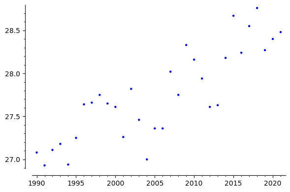
We wish to find the best fit line to the given set of data. Suppose the line is given by \(y=c+mx\text{,}\) then we wish to find \(a\) and \(b\) such that the line \(y=c+mx\) is best fit. Now what is meaning of "best fit". Suppose we consider the point \((x_i,y_i)\text{,}\) if it lies on \(c+mx\text{,}\) then \(y=c+mx_i\text{,}\) other wise \(|(c+mx_i)-y_i|\) is the error. We need to minimize this error for all the points. That is achieved by minimizing the sum of errors. Which is given by
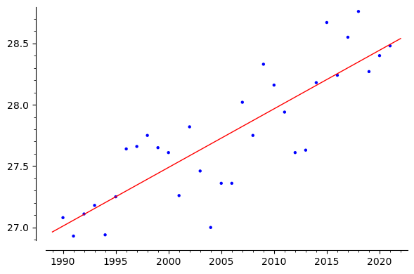
This means the slope of the fitted (regression line) is 0.0477584310854127 and the intercept is -68.0279710416216. Now we plot the fitted line along with the fitted line.
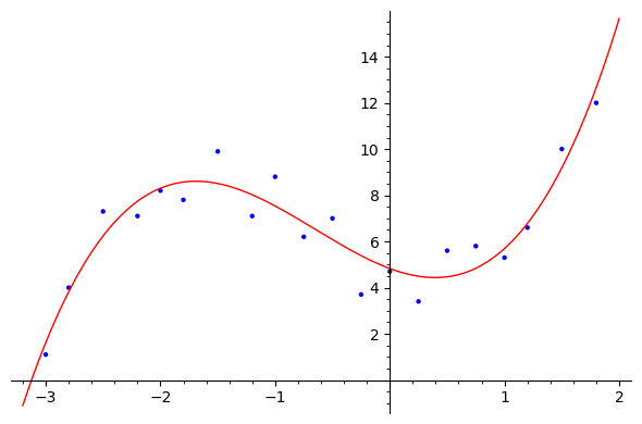
Suppose we are given a set of \(n\)-data points \((x_i y_i)\) and we wish to find the best fit polynomial curve of degree \(p\text{,}\) say, \(y=a_0+a_1x+a_2x^2+\cdots +a_px^p\text{,}\) with \(a_p\neq 0\text{.}\) In this case, the error term for \((x_i,y_i)\) from the the the curve \(y\) is \(|(a_0+a_1x_i+a_2x_i^2+\cdots +a_px_i^p)-y_i|\text{.}\) Thus the sum of the error square is
Weighted Least Squares (WLS) is an extension of the Ordinary Least Squares (OLS) method, allowing each observation to have a different weight based on its reliability. This is particularly useful when data points have unequal variances, a situation known as heteroscedasticity.
Consider the overdetermined system \(A\mathbf{x} \approx \mathbf{b}\text{,}\) where \(A \in \mathbb{R}^{m \times n}\) is the design matrix, \(\mathbf{x} \in \mathbb{R}^n\) is the vector of unknowns, and \(\mathbf{b} \in \mathbb{R}^m\) contains the observations. If the \(i\)-th observation has variance \(\sigma_i^2\text{,}\) the corresponding weight is \(w_i = \frac{1}{\sigma_i^2}\text{.}\) We define the diagonal weight matrix:
\begin{equation*}
W = \mathrm{diag}(w_1, w_2, \dots, w_m).
\end{equation*}