
Section 10.2 Applications of PCA

PCA, as mentioned earlier, is a dimensionality reduction techniques. It has numerous applications like, visualization of high dimensional data, facial recognition, computer vision, image compression, determining patterns in a data, data mining, bioinformatics, psychology, analyzing and forecasting stock data,etc. We mention, image compression as one of the applications.

Subsection 10.2.1 Image compression with PCA

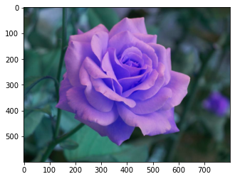
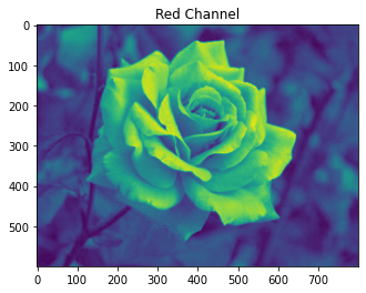
Similar to SVD, we can also compress the images using PCA. We take any image, first of all we separate the RBG channels of the images and apply PCA separately to red channel, green channel and blue channel. Next we take first \(k\) principal components and project the red, green and blue channel images and then combine the three channels to obtained the transformed image with \(k\) principal components.

Example 10.2.1.

Consider an image of a Rose as shown in the Figure 10.2.2 This image is of sinze \(600\times 800\times 3\) array.
Figure 10.2.2. Original Rose Image
The red green and blue channel images are shown in the Figures 10.2.3, Figure 10.2.4, Figure 10.2.5.
Figure 10.2.3. Red Channel
Figure 10.2.4. Green Channel
Figure 10.2.5. Blue Channel
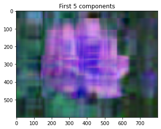
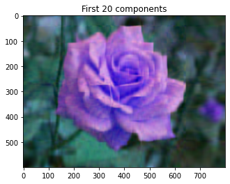
After applying PCA and taking first 5, 20 and 50 principal components and combining the three channels together we get the following approximate images as shown in the Figures 10.2.6, Figure 10.2.7, Figure 10.2.8, respectively. Each channel is of size \(600\times 800\text{.}\)
Figure 10.2.6. 5 components
Figure 10.2.7. 20 components
Figure 10.2.8. 50 components
We can see from the image, that 1st 50 components gives a very good approximation to the original image.

Subsection 10.2.2 Relation Between SVD and PCA

Consider a matrix \(X\) of size \(n\times d\text{.}\) We can apply SVD and PCA on \(X\text{.}\) Suppose the SVD of \(X\) is given by
\begin{equation*} X = U\Sigma V^T\text{.} \end{equation*}
Let \(U=[u_1~\ldots~ u_n]\) and \(V^T=\begin{bmatrix}v_1^T\\v_2^T\\\vdots\\v_d^T \end{bmatrix}\text{.}\) Then
\begin{equation*} X^TX = V\left( \Sigma^T\Sigma\right) V^T\text{.} \end{equation*}
The covariance matrix of \(X\) is \(\frac{1}{n-1}X^TX\text{.}\) This shows that \(S\) and \(X^TX\) are similar matrices. If \(\lambda_1,\ldots, \lambda_r\) are non zero eigenvalues of \(S\) and \(\sigma_1,\ldots, \sigma_r\) are singular values of \(X\text{.}\) Then they are related by the following relation
\begin{equation*} \sigma_i^2=(n-1)\lambda_i, i = 1, 2,\ldots, r\text{.} \end{equation*}
The relation \(X^TX = V\left( \Sigma^T\Sigma\right) V^T\) shows that right singular vectors are same as principal components. The left singular vectors are given by
\begin{equation*} u_i = \frac{1}{\sqrt{n-1}}Xv_i\text{.} \end{equation*}

Subsection 10.2.3 Exercise Set

Checkpoint 10.2.9.

Find the singular values Decomposition of the following matrices.
(a) \(\begin{bmatrix}-2 \amp 2 \\ 1 \amp 1 \end{bmatrix}\text{,}\)(b) \(\begin{bmatrix}1 \amp 1 \\ 0 \amp 1 \\1 \amp 0 \end{bmatrix}\text{,}\) (c) \(\begin{bmatrix}-1 \amp 1 \\ -1 \amp 1\\2 \amp -2 \end{bmatrix}\text{,}\) (d) \(\begin{bmatrix}1 \amp 1 \\ -3 \amp -3 \end{bmatrix}\text{,}\) (e) \(\begin{bmatrix}1 \amp -1 \amp 0 \\ 0 \amp 0 \amp 1\\-1 \amp 1\amp 0 \end{bmatrix}\)

Checkpoint 10.2.10.

Use SVD to find generalized inverse of the following matrices:
(a) \(\begin{bmatrix}1 \amp 1 \\ -3 \amp -3 \end{bmatrix}\text{,}\) (b) \(\begin{bmatrix}1 \amp -1 \amp 0 \\ 0 \amp 0 \amp 1\\-1 \amp 1\amp 0 \end{bmatrix}\text{,}\) (c) \(\begin{bmatrix}1 \amp 0 \amp -1\\-1 \amp 0 \amp 1\\0 \amp 1 \amp 0 \end{bmatrix}\text{.}\)

Checkpoint 10.2.11.

Use the generalized inverse from the SVD to find the least square solution of the system of linear equations \(Ax=b\) where
\begin{equation*} \begin{bmatrix}1 \amp 2 \\ -1 \amp 1\\ 2 \amp 1\\ 2 \amp -1\\1 \amp 1 \end{bmatrix} , b=\begin{bmatrix}2 \amp 1 \amp -2 \amp 1 \amp 3 \end{bmatrix}\text{.} \end{equation*}

Checkpoint 10.2.12.

Find the principal components of the matrix
\begin{equation*} \begin{bmatrix}3 \amp -4 \amp 7 \amp 1 \amp -4 \amp -3\\7 \amp -6 \amp 8 \amp -1 \amp -1 \amp 7 \end{bmatrix} \end{equation*}
What percentage of the variation in the data is explained by the first principal component.