Eigenvalues and Eigenvectors

Section 5.1 Eigenvalues and Eigenvectors

In this chapter, we extend our study of linear transformations to the concepts of eigenvalues and eigenvectors, essential for understanding how certain vectors retain their direction under transformation—merely being scaled by a scalar factor.

🔗

These ideas lie at the heart of many core themes in linear algebra. In particular, they lay the mathematical foundation for:

🔗

Diagonalization of matrices—simplifying linear transformations to their most transparent form.

🔗
Dynamical systems, including Markov chains and population models, where long-term behavior is driven by dominant eigenvalues.

🔗
Methods for solving systems of linear differential equations via eigen-decomposition.

🔗
Dimensional reduction techniques such as Principal Component Analysis (PCA), where eigenvalues guide us in identifying principal directions.

🔗
Web algorithms such as PageRank, leveraging eigenvectors to reveal stable structures.

🔗

Throughout the chapter, we will combine conceptual insight with computational exploration using SageMath, helping you see not only “what” eigenvalues and eigenvectors are, but also “how” to compute them effectively and “where” they matter in applications that span mathematics and applied sciences.

🔗

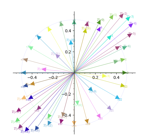
Subsection 5.1.1 Eigenvalues and Eigenvectors

Suppose \(T\) is a linear map from a vector space \(V\) to itself. For a given \(v\text{,}\) \(T(v)\) is a vector in \(V\text{.}\) Look the Figure 5.1.1 in which image of vectors \(v_1,\ldots v_{24}\) under the linear map \(T(x,y)=(x/2+y,x+y/2)\) are shown. Notice that \(v_3\) and \(T(v_3)\) are parallel, similarly \(v_{21}\) and \(T(v_{21})\) are parallel.

Figure 5.1.1. Image of vectors under \(T(x,y)=(x/2+y,x+y/2).\)
🔗

You can also observe that \(v_{15}\) and \(T(v_{15})\) are parallel, but this this expected as \(v_{15}=-v_3\text{.}\) Similarly \(v_{9}\) and \(T(v_{9})\) are parallel. Such vectors are called eigenvectors of \(T\text{.}\) In particular, \(v\) and \(T(v)\) are parallel, then \(T(v)=\lambda v\) for some \(\lambda\in \R\text{,}\) such a \(\lambda\) is called the eigenvalue corresonidng to eigenvector \(v\text{.}\) What happens if \(v=0\text{?}\)

🔗

You can also explore the same while rotating a vector \(v\) and observing what happens to its image using the interactive diagram below (see Figure 5.1.2).

🔗

Figure 5.1.2. Exploration of eigenvectors

🔗

These exploration leads to the following definition of eigenvector and eigenvalues.

🔗

Definition 5.1.3. Eigenvalues and Eigenvectors.

Let \(T\) be a linear transformation from \(\mathbb{R}^n\to \R^n\text{.}\) A real number (scalar) is called an eigenvalue of \(T\) if there exists a non zero vector \(v\in \R^n\) (called an eigenvector corresponding to eigenvalue \(\lambda\)) if \(T(v)=\lambda v\text{.}\) That is, if \(T(v)\) is parallel to \(v\text{.}\)

🔗

Thus if \(T(v)=\lambda v\text{,}\) then \({\lambda I-T}(v)=0\text{,}\) where \(I\) is identity transformation on \(V\text{.}\)

🔗

If \(A\) is an \(n\times n\) real matrix matrix, then we know that \(T_A(x)=Ax\) is a linear transformation induced by \(A\text{.}\) We can define eigenvalue of \(A\) as eigenvalue of \(T_A\text{.}\) In particular, real number is called an eigenvalue of \(A\) if there exists a non zero vector \(v\in \R^n\) (called an eigenvector corresponding to eigenvalue \(\lambda\)) if \(Av=\lambda v\text{.}\)

🔗

Example 5.1.4.

Let \(A=\left(\begin{array}{rr} 1 \amp 2 \\ -1 \amp 4 \end{array} \right)\text{.}\) Consider a vector \(u=\begin{pmatrix}1\\1 \end{pmatrix}\text{.}\) Then \(Au=\begin{pmatrix}3\\3 \end{pmatrix} =3\begin{pmatrix}1\\1 \end{pmatrix} =3u\text{.}\) Hence \(u\) is an eigenvector and \(\lambda = 3\) is an eigenvalue.

🔗

Consider \(v=\begin{pmatrix}2\\1 \end{pmatrix}\text{.}\) Then it is easy to check that \(Av=\begin{pmatrix}4\\2 \end{pmatrix} =2\begin{pmatrix}2\\1 \end{pmatrix}\text{.}\) Hence \(v\) is also an eigenvector and \(\lambda = 2\) is an eigenvalue.

🔗

Example 5.1.5.

If \(T\) is an identity transformation from \(\R^n\to \R^n\text{,}\) then every nonzero vector is an eigenvector corresponding the eiegenvalue 1. The same is true for \(n\times n \) identity matrix.

🔗

Example 5.1.6.

Consider the matrix of rotation \(R_\theta\) in anti-clock wise by an angle \(\theta\neq n\pi\) for \(n\in \Z\text{.}\) Then it is easy to see that \(R_\theta\) does not have an eigenvector. Thus not all square matrices have eigenvectors.

🔗

Remark 5.1.7.

If \(\lambda\) is an eigenvalue of \(A\) with corresponding eigenvector \(v\neq 0\text{.}\) Then any scalar multiple of \(v\) is also an eigenvector corresponding to the same eigenvalue \(\lambda\text{.}\)

🔗

If \(Av=\lambda v\text{,}\) then

\begin{equation*} A(\alpha v)=\alpha Av=\alpha \lambda v =\lambda (\alpha ). \end{equation*}

🔗

Let us analyze the notion of eigenvalues and eigenvector. If \(v\) is a eigenvector corresponding to an eigenvalue \(\lambda\text{.}\) Then \(Av=\lambda v\text{.}\) This implies \((\lambda I-A)v=0\text{,}\) where \(I\) is \(n\times n\) identity matrix. This means that the homogeneous system \((\lambda I-A)x=0\) has a non zero solution, namely \(v\text{.}\) Hence \(\det{(\lambda I-A)}=0\text{.}\) Notice that \(\det(A-\lambda I)\) is a polynomial (called the characteristic polynomial of \(A\)) of degree \(n\) in \(\lambda\text{.}\) Thus if \(Av=\lambda v\text{,}\) then \(\lambda\) is a root of the the characteristic polynomial \(\det(A-\lambda I)\text{.}\) By fundamental theorem of algebra an \(n\times n\) real matrix can have at most \(n\) real eigenvalues. The equation \(\det(A-\lambda I)=0\) is called characteristic equation of \(A\text{.}\)

🔗

We can write \(\det(A-\lambda I)=0\) as

\begin{equation*} \det(A-\lambda I)=\lambda^n-c_1\lambda^{n-1}+c_2\lambda^{n-2}-\cdots+(-1)^nc_n=0. \end{equation*}

If \(\lambda_1,\ldots, \lambda_n\) are roots of the characteristics equation, then using the theory of equations one can show that

\begin{align} \lambda_1+\cdots+\lambda_n\amp = c_1={\rm trace}(A)\tag{5.1.1}\\ \lambda_1\lambda_2+\cdots +\lambda_{n-1}\lambda_n \amp = c_2\tag{5.1.2}\\ \vdots \amp \notag\\ \lambda_1\lambda_2\cdots\lambda_n \amp = c_n = \det(A)\text{.}\tag{5.1.3} \end{align}

🔗

Thus we have the following.

🔗

Theorem 5.1.8.

Let \(A\) be an \(n\times n\) real matrix. Then (i) the sum of eigenvalues of \(A\) is the trace of \(A\) and (ii) the product of eigenvalues is the determeninat of \(A\text{.}\)

🔗

Example 5.1.9.

Let \(A = \begin{pmatrix}1 \amp 1 \amp 1\\ 1 \amp 1 \amp 1\\1 \amp 1 \amp 1 \end{pmatrix}\text{.}\) What are eigenvalues and eigenvectors of \(A\text{?}\)

🔗

Note that \(Ae_1=Ae_2=Ae_3=e_1+e_2+e_3\text{.}\) This means \(A(e_1+e_2+e_3)=3(e_2+e_2+e_3)\text{.}\) Hence \(3\) is an eigenvalue and \(e_1+e_2+e_3=\begin{pmatrix}1 \\1\\1 \end{pmatrix}\) is an eigenvectors w.r.t. eigenvalue 3.

🔗

Also \(A(e_1-e_2)=0\text{.}\) Hence \(0\) is an eigenvalue and \(e_1-e_2=\begin{pmatrix}1 \\-1\\0 \end{pmatrix}\) is an eigenvector corresponding to the eigenvalue 0. Also, \(e_1-e_3\) and \(e_2-e_3\) are also eigenvectors corresponding to the eigenvalue 0.

🔗

Note that in this example, we are able to find eigenvalues and eigenvectors by inspection and without going through characteristic polynomials.

🔗

What will be generalization of this example?

🔗

Example 5.1.10.

Let \(A = \begin{pmatrix}1 \amp t \amp t\\ t \amp 1 \amp t\\t \amp t \amp 1 \end{pmatrix}\text{.}\) What are eigenvalues of \(A\text{?}\)

🔗

The trace of \(A\) is 3. The \(\det{(A)}=2t^3 - 3t^2 + 1=(2t + 1)(t - 1)^2\text{.}\) Since sum of eigenvalues is 3 and the product of eigenvalues is \(\det{(A)}\text{,}\) it is easy to guess that \(\lambda_1 =2t+1\text{,}\) \(\lambda_2=\lambda_3=1-t\) are eigenvalues of \(A\text{.}\)

🔗

We can adopt a procedure similar to Example 5.1.10 to show that \(e_1+e_2+e_3\) is an eigenvector corresponding to the eigenvalue \(1+2t\text{.}\) Similarly, \(e_1-e_2,e_2-e_3, e_1-e_3\) are eigenvectors corresponding to the eigenvalue \(1-t\text{.}\)

🔗

Example 5.1.11.

Let \(A=\begin{pmatrix}1\amp 2\amp -2\\1\amp 1\amp 1\\1\amp 3\amp -1 \end{pmatrix}\text{.}\) Find eigenvalues and corresponding eigenvector of \(A\text{.}\)

🔗

We have

\begin{equation*} \det(A-\lambda I)=\begin{vmatrix}1-\lambda\amp 2\amp -2\\ 1\amp 1-\lambda\amp 1\\1\amp 3\amp -1-\lambda \end{vmatrix}=\lambda^3-\lambda^2-4\lambda+4\text{.} \end{equation*}

It is easy to see that characteristic polynomial \(\det(A-\lambda I)\) has roots \(\lambda=1, \lambda=-2, \lambda=2\text{.}\) Thus \(A\) has eigenvalues \(1, -2, 2\text{.}\)

🔗

Let us find eigenvectors with respect to the eigenvalue \(\lambda=1\text{.}\) Let \(v=\begin{pmatrix}x_1\\x_2\\x_3 \end{pmatrix}\) be an eigenvector corresponding to \(\lambda=1\text{.}\) Then \(Av=\lambda v=v\text{.}\) That is,

\begin{equation*} \begin{pmatrix}1\amp 2\amp -2\\1\amp 1\amp 1\\1\amp 3\amp -1 \end{pmatrix} \begin{pmatrix}x_1\\x_2\\x_3 \end{pmatrix} =\begin{pmatrix}x_1\\x_2\\x_3 \end{pmatrix}\text{.} \end{equation*}

🔗

This gives a system of linear equations

\begin{equation*} x_1+2x_2-2x_3=x_1; x_1+x_2+x_3=x_2; x_1+3x_2-x_3=x_3 \end{equation*}

🔗

Solving the above system, we get \(x_1=-x_2, x_2=x_3\text{.}\) Thus \(v=\begin{pmatrix}\alpha\\-\alpha\\-\alpha \end{pmatrix}\) for \(\alpha\in \R\) is an eigenvector. In particular, \(v=\begin{pmatrix}1\\-1\\-1 \end{pmatrix}\) is an eigenvector of \(A\) corresponding to \(\lambda=1\text{.}\)

🔗

Similarly show that \(\begin{pmatrix}0\\1\\1 \end{pmatrix}\) is an eigenvector of \(A\) corresponding to \(\lambda=2\) and \(\begin{pmatrix}8/7\\-5/7\\1 \end{pmatrix}\) is an eigenvector of \(A\) corresponding to \(\lambda=-2\)

🔗

Example 5.1.12.

Let \(\begin{pmatrix}0\amp 1\\-1\amp 0 \end{pmatrix}\text{.}\) Find eigenvalues and corresponding eigenvector of \(A\text{.}\)

🔗

The characteristic equation of \(A\) is given by \(\det(A-\lambda I)=\begin{vmatrix}-\lambda\amp 1\\-1\amp -\lambda\end{vmatrix}=\lambda^2+1\text{.}\) Hence eigenvalues of \(A\) are \(\lambda=\pm i\text{.}\)

🔗

Let us find eigenvectors with respect to the eigenvalue \(\lambda=i\text{.}\) Let \(v=\begin{pmatrix}x_1\\x_2 \end{pmatrix}\) be an eigenvector corresponding to \(\lambda=i\text{.}\) Then \(Av=\lambda v=i v\text{.}\) That is,

\begin{equation*} \begin{pmatrix}0\amp 1\\-1\amp 0 \end{pmatrix} \begin{pmatrix}x_1\\x_2 \end{pmatrix} =\begin{pmatrix}i x_1\\ ix_2 \end{pmatrix} \Longrightarrow \begin{pmatrix}x_2\\-x_1 \end{pmatrix} =\begin{pmatrix}i x_1\\ ix_2 \end{pmatrix}\text{.} \end{equation*}

🔗

Now it is easy to see that \(v=\begin{pmatrix}1\\ i \end{pmatrix}\) is an eigenvector of \(A\) corresponding to \(\lambda=i\text{.}\) Similarly one can show that \(v=\begin{pmatrix}1\\ -i \end{pmatrix}\) is an eigenvector of \(A\) corresponding to \(\lambda=-i\text{.}\)

🔗

Note that in the above example, \(A\) is a real matrix but its eigenvalues and eigenvectors are complex.

🔗

Example 5.1.13.

Suppose \(A\) is a diagonal matrix, then eigenvalues of \(A\) are diagonal entries.
🔗

🔗
Suppose \(A\) is an \(n\times n\) triangular (upper /lower) matrix, the eigenvalues of \(A\) are the main diagonal entries.
🔗

🔗

🔗

Reading Questions Reading Questions

1.

Let \(A\) an \(n\times n\) real matrix and \(\lambda\in \R\) be an eigenvalue of \(A\text{.}\) Then

\begin{equation*} E_\lambda = \{x\in \R^n: Ax=\lambda x\} \end{equation*}

is a subspace of \(\R^n\text{.}\)

🔗

2.

\(E_\lambda\) is the kernel of \(A-\lambda I\text{.}\)

🔗

Hint.

Let \(v_1,v_2 \in E_\lambda\text{.}\) Then

\begin{equation*} A(v_1+v_2)=Av_1+Av_2=\lambda v_1+\lambda_v2= \lambda(v_1+v_2). \end{equation*}

\begin{equation*} \text{for } \alpha\in R, A(\alpha v)=\alpha Av=\alpha \lambda v=\lambda(\alpha v). \end{equation*}

🔗

Definition 5.1.14. Eigenspace.

Let \(A\) an \(n\times n\) real matrix and \(\lambda\in \R\) be an eigenvalue of \(A\text{.}\) Then

\begin{equation*} E_\lambda = \{x\in \R^n: Ax=\lambda x\} \end{equation*}

the collection of all eigenvectors of \(A\) corresponding to \(\lambda\) is a subspace of \(A\text{,}\) called the eigenspace of \(A\). The dimension of \(E_\lambda\) is called the geometric multiplicity of \(A\text{.}\)

🔗

Let \(x\) be a enigenvector correspnding to the eigenvalue \(\lambda\text{.}\) Let the characteristic polynomila of \(A\) splits as

\begin{equation*} p(x)=\det{(x I -A)}=(x-\lambda_1)^{m_1}(x-\lambda_2)^{m_2}\cdots (x-\lambda_k)^{m_k}. \end{equation*}

Then \(\lambda_i\) are eigenvalue of \(A\) with multiplicity \(m_i\text{,}\) called the algebraic multiplicity of \(\lambda_i\text{.}\)

🔗

We mention, the following theorem without proof at this stage. We shall see the proof later.

🔗

Theorem 5.1.15.

Geometric multiplicity of an eigenvalue is always less than or equals to its algebraic multiplicity. That is, if \(m\) is the geometric multiplicity of \(\lambda\) then \(\dim{(E_\lambda)} \leq m\text{.}\)

🔗

Checkpoint 5.1.16.

The geometric multiplicity of an eigenvalue \(\lambda\) is the nullity of \(A-\lambda I\) which is the dimension of null space of \(A-\lambda I\text{.}\)

🔗

Example 5.1.17.

Consider the matrix \(A=\begin{pmatrix}-1\amp 1 \amp 0\\0 \amp -1 \amp 1\\0 \amp 0 \amp -1 \end{pmatrix}\text{.}\) It is easy to check that \(\det{(xI-A)}=(x+1)^3\text{.}\) That is, \(A\) has only one eigenvalue of \(\lambda =-1\) of algebraic multiplicity 3. It is easy to see that \(e_3=(0,0,1)\) is an eigenvector corresponding to \(\lambda=-1\text{.}\) We have

\begin{equation*} A -\lambda I = \begin{pmatrix}0\amp 1 \amp 0\\0 \amp 0 \amp 1\\0 \amp 0 \amp 0 \end{pmatrix}\text{.} \end{equation*}

Since the rank of \(A-\lambda I\) is 2. By rank-nullity theorem, nullity of \(A -\lambda I\) is 1. Hence the geometric multiplicity of \(\lambda\) is 1 where as its algebraic multiplicity is 3.

🔗

We list the following properties of eigenvalues and eigenvectors without proof.

🔗

Theorem 5.1.18. Properties of Eigenvalues and Eigenvectors.

\(A\) and \(A^T\) have the same eigenvalues.
🔗

🔗
If \(\lambda\) is an eigenvalue of \(A\text{,}\) then \(\alpha \lambda\) is an eigenvalue of \(\alpha A\text{.}\)
🔗

🔗
If \(\lambda\) is an eigenvalue of \(A\text{,}\) then \(\lambda^2\) is an eigenvalue of \(A^2\text{.}\) In general, \(\lambda^k\) is an eigenvalue of \(A^2\) for any \(k\in \N\text{.}\)
🔗

🔗
If \(\lambda\) is an eigenvalue of a non singular matrix \(A\text{,}\) then \(1/ \lambda\) is an eigenvalue of \(A^{-1}\text{.}\)
🔗

🔗
If \(\lambda\) is an eigenvalue of \(A\text{,}\) then \(\lambda-k\) is an eigenvalue of \(A-kI\) for any scalar \(k\text{.}\)
🔗

🔗
If \(\lambda\) is an eigenvalue of \(A\) and \(p(x)=c_0+c_cx+c_2x^2+\cdots c_kx^k\) is a polynomial in \(x\text{,}\) then \(p(\lambda)\) is an eigenvalue of \(p(A)=c_0I+c_cA+c_2A^2+\cdots c_kA^k\text{.}\)
🔗

🔗
Two matrices \(A\) and \(B\) are called similar if there exists a matrix \(P\) such that \(B=P^{-1}AP\text{.}\) Similar matrices have same eigenvalues.
🔗

🔗
If \(\lambda_1\) and \(\lambda_2\) are distinct eigenvalues of \(A\) then eigenvectors \(v_1\) and \(v_2\) corresponding to \(\lambda_1\) and \(\lambda_2\) are linearly independent. Can you generalize this?
🔗

🔗
If \(T\) is a linear transformation from \(\R^n\to \R^m\text{.}\) Fix a basis \(\beta\) of \(\R^n\text{.}\) Let \(A=[T]_\beta\) be the matrix of \(T\) with respect to \(\beta\text{.}\) Then \(A\) and \(T\) have the same eigenvalues. Furthermore, eigenvalues of \(T\) are independent of the basis.
🔗

🔗

🔗

Proof.

Proof of Item 1.

🔗

Follows from \(\det{A^T}=\det{A}\text{.}\) For \(\det{(xI-A)^T}=\det{(xI-A)}.\)

🔗

Proof of Item 2.

🔗

\(A(\alpha v)=\alpha Av =\alpha\lambda v=\lambda(\alpha v)\text{.}\)

🔗

Proof of Item 3.

🔗

\(A^2(v)=A(Av) =A(\lambda v)=\lambda(\lambda v)=\lambda^2 v\text{.}\)

🔗

Proof of Item 4.

🔗

\(A(v)=\lambda v\implies \frac{1}{\lambda}v=A^{-1}v\text{.}\)

🔗

Proof of Item 5.

🔗

\((A-kI)(v)=Av -\lambda v =\lambda v-\lambda v=(\lambda-k)v\text{.}\)

🔗

Proof of Item 6.

🔗

\begin{equation*} p(A)v=c_0v+c_c\lambda v+c_2\lambda^2v+\cdots c_k\lambda^kv=p(\lambda). \end{equation*}

🔗

Proof of Item 7.

🔗

Since

\begin{equation*} \det(\lambda I-A) = \det\left(P(\lambda I-A)P^{-1}\right), \end{equation*}

the eigenvalues of \(A\) and \(PAP^{-1}\) are same.

🔗

Proof of Item 8.

🔗

Let \(\lambda_1\) and \(\lambda_2\) be with distict eigenvalues of \(A\) corresponding to the eignevectors, \(v_1\) and \(v_2\) respectively. Let \(\alpha_1\) and \(\alpha_2\) be scalars such that \(\alpha_1v_+\alpha_2 v_2=0.\text{.}\) Applying \(A\) both sides we have \(\alpha_1\lambda_1v_1+\alpha_2\lambda_2 v_2=0\text{.}\) Mutliplying the 1st equation both sides by \(\lambda_1\) both side and subtracting from the equation 2nd equation we get \(\alpha_2(\lambda_2-\lambda_1)v_2=0\text{.}\) Since \(v_2\neq 0 \text{,}\) and \(\lambda_1\neq \lambda_2\text{,}\) we have \(\alpha_2=0\text{.}\) Similarly, \(\lambda_1=0\text{.}\)

🔗

We have the following generalization. If \(v_i\) for \(i=1,\ldots, k\) are eigenvvectors with respect to distinct eigenvalues \(\lamabda_i\) for \(i=1,\ldots, k\) respectively, then \(v_1,\ldots, v_k\) are linearly independent. The prove this follows from induction on \(k\text{.}\)

🔗

Proof of Item 9.

🔗

Since \(T\colon \R^n\to \R^n\) is a linear transformation, it can be written as \(T(x)=M\text{,}\) where \(M\) is the matrix of \(T\) with respect to the standard basis of \(\R^n\) and that eigenvalues of \(T\) are same as eigenvalues of \(A\text{.}\) Then \(A\) and \(M\) are similar matrices. Hence they have the same eigenvalues.

🔗

Example 5.1.19.

Let \(A=\begin{pmatrix}1\amp 2\amp -2\\1\amp 1\amp 1\\1\amp 3\amp -1 \end{pmatrix}\) and \(B=A^3-3A+I\text{.}\) Let us find eigenvalues of \(B\text{.}\)

🔗

It is easy to the characteristic polynomial of \(A\) is given by \(\lambda^3-\lambda^2-4\lambda+4\) and \(\lambda=-2, 1, 2\text{.}\) Then eigenvalues of \(B\) are given by

\begin{equation*} \{(-2)^3-3\times (-2)+1, 1^3-3\times 1+1, 2^3-3\times (2)+1\} =\{-1, -1, 3\} \end{equation*}

🔗

In genegarl, let \(f(x)=\alpha_0+\alpha_1 x+\alpha_2 x^2+\cdots+\alpha_kx^k\) be a polynomial of degree \(k\) and \(A\) be an \(n\times n\) real matrix. Then we can define \(f(A)=\alpha_0 I+\alpha_1 A+\alpha_2 A^2+\cdots+\alpha_k A^k\text{.}\) If \(\lambda\) is an eigenvalue of \(A\text{,}\) theh \(f(\lambda)\) is an eigenvalue of \(f(A)\text{.}\)

🔗

Theorem 5.1.20. Cayley-Hamilton Theorem.

Every square matrix satisfies its characteristic equation. That is, if \(p(x)=0\) is characteristic equation of \(A\text{,}\) then \(p(A)=0\text{.}\)

🔗

Proof.

The proof is an application of the formula

\begin{equation*} A\text{adj}(A)=\det{(A)}I \end{equation*}

where \(\det{(A)}\) is the adjugate of a \(A\) and is defined as the transpose of its cofactor matrix.

🔗

We apply the adjugate formula to the matrix \(\lambda I-A\text{.}\) Hence we have

\begin{equation} (\lambda I-A)\text{adj}(tI-A)=\det(\lambda I-A)\,I = p(\lambda)\,I. \tag{5.1.4} \end{equation}

Note that adjugate matrix \(\text{adj}(\lambda I-A)\) is an \(n\times n\) matrix whose entries are polynomials in \(\lambda\) of degree at most \(n-1\text{.}\) Hence we may write

\begin{equation*} \text{adj}( \lambda I-A)=\sum_{k=0}^{n-1} C_k \lambda^k, \end{equation*}

where \(C_k's\) are matrices with real entries. Hence by (5.1.4), we have

\begin{equation} (\lambda I-A) \left(\sum_{k=0}^{n-1} C_k \lambda^k\right) = A^n+a_{n-1}A^{n-1}+a_1A+a_0I.\tag{5.1.5} \end{equation}

Now comparing the coefficients of power of \(\lambda\text{,}\) we get

\begin{align*} C_{n-1}\amp = I\\ C_{n-2}-AC_{n-1}\amp = a_{n-1}I\\ C_{n-3}-AC_{n-2}\amp = a_{n-2}I\\ \amp \vdots\\ C_{0}-AC_{1}\amp = a_{1}I\\ -AC_{0}\amp = a_{0}I \end{align*}

Multiplying the first equation by \(A^n\text{,}\) the second equation by \(A^{n-1}\text{,}\) the second last equation by \(A\) and the last equation by \(I\) and additing, we get the desired result.

🔗

Example 5.1.21.

Let \(A=\begin{pmatrix}1\amp 2\amp -2\\1\amp 1\amp 1\\1\amp 3\amp -1 \end{pmatrix}\text{.}\) From Example 5.1.11, the characteristic polynomial of \(A\) is given by \(p(x)=\det{x I -A}=x^3-x^2-4x+4\text{.}\) We have \(A^2=\left(\begin{array}{rrr} 1 \amp -2 \amp 2 \\ 3 \amp 6 \amp -2 \\ 3 \amp 2 \amp 2 \end{array} \right)\) and \(A^3=\left(\begin{array}{rrr} 1 \amp 6 \amp -6 \\ 7 \amp 6 \amp 2 \\ 7 \amp 14 \amp -6 \end{array} \right)\text{.}\) Hence

\begin{align*} p(A) =\amp A^3-A^2-4A+4I\\ =\amp \left(\begin{array}{rrr} 1 \amp 6 \amp -6 \\ 7 \amp 6 \amp 2 \\ 7 \amp 14 \amp -6 \end{array} \right)- \left(\begin{array}{rrr} 1 \amp -2 \amp 2 \\ 3 \amp 6 \amp -2 \\ 3 \amp 2 \amp 2 \end{array} \right)\\ \amp -4\begin{pmatrix}1\amp 2\amp -2\\1\amp 1\amp 1\\1\amp 3\amp -1 \end{pmatrix} +4\begin{pmatrix}1\amp 0\amp 0\\0\amp 1\amp 0\\ 0\amp 0\amp 1 \end{pmatrix}\\ =\amp \begin{pmatrix}0\amp 0\amp 0\\0\amp 0\amp 0\\ 0\amp 0\amp 0 \end{pmatrix} \text{.} \end{align*}

🔗

Hence \(A\) satisfies its characteristic equation.

🔗

It is easy to check that \(\det{(A)}=-4\text{,}\) hence \(A\) is non singular. Since \(A^3-A^2-4A+4I=0\text{,}\) multiplying both sides by its inverse, we get \(A^2-A+4I+4A^{-1}=0\text{.}\) Hence

\begin{equation*} A^{-1}=-\frac{-1}{4}A^2+\frac{1}{4}A+I=\left(\begin{array}{rrr} 1 \amp 1 \amp -1 \\ -\frac{1}{2} \amp -\frac{1}{4} \amp \frac{3}{4} \\ -\frac{1}{2} \amp \frac{1}{4} \amp \frac{1}{4} \end{array} \right)\text{.} \end{equation*}

🔗

We can also find higher powers of a matrix, using the Cayley-Hamilton theorem. For example multiplying by \(A\) to the equation, \(A^3-A^2-4A+4I=0\text{,}\) we get \(A^4-A^3-4A^2+4A=0\text{,}\) from this we have

\begin{equation*} A^4 = A^3+4A^2-4A=\left(\begin{array}{rrr} 1 \amp -10 \amp 10 \\ 15 \amp 26 \amp -10 \\ 15 \amp 10 \amp 6 \end{array} \right)\text{.} \end{equation*}

🔗

Can you find \(A^5\text{?}\)

🔗

Checkpoint 5.1.22.

(i) Consider the matrix \(A = \begin{pmatrix}3 \amp -2 \\-4\amp 3 \end{pmatrix}\text{.}\) Show that \(A\) satisfies its characteristics equation. Hence find \(A^{-1}, A^3, A^4\text{.}\)

🔗

(i) Consider the matrix \(A = \begin{pmatrix}1 \amp 0 \amp 0 \\ -4 \amp -3 \amp 4 \\ -2 \amp -2 \amp 3 \end{pmatrix}\text{.}\) Show that \(A\) satisfies its characteristics equation. Hence find \(A^{-1}, A^4, A^5\text{.}\)

🔗

Definition 5.1.23. Spectral Radius.

Let \(A\) an \(n\times n\) and \(\lambda_i\) for \(1\leq i\leq n\) be eigenvalues of \(A\) then the spectral radius of \(A\) is define as \(\rho(A):=\displaystyle\max_{1\leq i\leq n}\{ |\lambda_i| \}\text{.}\)

🔗

Example 5.1.24.

Let \(A= \begin{pmatrix}0 \amp -1\\1 \amp 0 \end{pmatrix}\text{.}\) Then the characteristics polynomial of \(A\) is \(\det{(xI-A)}=x^2+1\text{.}\) Hence \(x=\{i,-i\}\) are roots of the characteristic polynomial. Hence \(i\) and \(-i\) are eigenvalues of \(A\text{.}\) Hence

\begin{equation*} \rho(A) = \max\{|i|,|-i|\}=1\text{.} \end{equation*}

🔗

Example 5.1.25.

Consider the matrix \(A=\left(\begin{array}{rrr} 4 \amp -3 \amp 0 \\ 3 \amp 4 \amp 0 \\ 5 \amp 10 \amp 10 \end{array} \right)\text{.}\) Then the characteristics polynomial of \(A\) is \(\det{xI-A}=x^{3} - 18 x^{2} + 105 x - 250\text{.}\) Which has roots, \(10, 3-4i,3+4i\text{.}\) Hence

\begin{equation*} \rho(A) = \max\{10,|3-4i|,|3+4i\}=10\text{.} \end{equation*}

🔗

Checkpoint 5.1.26.

Find the spectral radius of \(\left(\begin{array}{rr} 2 \amp -3 \\ 3 \amp 2 \end{array} \right), \left(\begin{array}{rrr} 2 \amp 3 \amp 1 \\ -3 \amp 2 \amp 2 \\ 0 \amp 0 \amp 2 \end{array} \right)\) and \(\left(\begin{array}{rrr} 2 \amp 3 \amp 1 \\ 3 \amp 2 \amp 2 \\ 0 \amp 0 \amp 1 \end{array} \right)\text{.}\)

🔗

Definition 5.1.27. Positive definite matrix.

Let \(A\) be an \(n\times n\) symmetric matrix. Then \(A\) is said to be positive definite if \(x^TAx\gt 0\) for all \(x\in \R^n\setminus \{0\}\) and \(x^TAx=0\) if and only if \(x=0\text{.}\) \(A\) is called negative definite if \(-A\) is positive definite.

🔗

Example 5.1.28.

Let \(A=\begin{pmatrix}1\amp 2\\2\amp 5 \end{pmatrix}\text{.}\) Let \(x=\begin{pmatrix}x_1\\x_2 \end{pmatrix}\text{.}\) Then

\begin{align*} x^TAx=\amp \begin{pmatrix}x_1\amp x_2 \end{pmatrix} \begin{pmatrix}1\amp 2\\2\amp 5 \end{pmatrix} \begin{pmatrix}x_1\\x_2 \end{pmatrix}\\ =\amp \begin{pmatrix}x_1\amp x_2 \end{pmatrix} \begin{pmatrix}x_1+2x_2\\2x_1+5x_2 \end{pmatrix} \\ =\amp x_1^2+4x_1x_2+5x_2^2=(x_1+2x_2)^2+x_2^2\text{.} \end{align*}

🔗

Clearly \(x^TAx>0\) for all non zero vector \(x\) and \(x^TAx=0\) if and only if \(x=0\text{.}\) Hence \(A\) is positive definite.

🔗

Example 5.1.29.

Let \(A=\begin{pmatrix}0\amp 1\\1\amp 0 \end{pmatrix}\text{.}\) Let \(x=\begin{pmatrix}x_1\\x_2 \end{pmatrix}\text{.}\) Then

\begin{equation*} x^TAx=\begin{pmatrix}x_1\amp x_2 \end{pmatrix} \begin{pmatrix}0\amp 1\\1\amp 0 \end{pmatrix} \begin{pmatrix}x_1\\x_2 \end{pmatrix} = \begin{pmatrix}x_1\amp x_2 \end{pmatrix} \begin{pmatrix}x_2\\x_1 \end{pmatrix} =2x_1x_2 \end{equation*}

🔗

Thus if \(x=\begin{pmatrix}1\\-1 \end{pmatrix}\) then \(x^TAx=-2\lt 0\text{.}\) Hence it is not a positive definite. Its easy to see that \(A\) is also not negative definite.

🔗

Checkpoint 5.1.30.

If \(A\) is a positive definite matrix then all its eigenvalues are positive.

🔗

Checkpoint 5.1.31.

If \(A\) is a negative definite matrix then all its eigenvalues are negative.

🔗

We have the following result about positive definite matrices known as Sylvester’s criterion. It allows us to determine if a given matrix in positive definite using the leading principal minors of the matrix.

🔗

The leading principal minors of a matrix \(A\) are \({\rm det}(A)\) and the minors obtained by successively removing the last row and the last columns. That is, the leading principal miniors of a matrix \(A\) are

\begin{equation*} \Delta_1 =a_{11}, \Delta_2 =\begin{vmatrix}a_{11} \amp a_{12}\\a_{21} \amp a_{22}\end{vmatrix}, \Delta_3= \begin{vmatrix}a_{11} \amp a_{12} \amp a_{13}\\a_{21} \amp a_{22} \amp a_{23}\\a_{31} \amp a_{32}\amp a_{33}\end{vmatrix}, \cdots, \Delta_n ={\rm det}{(A)}\text{.} \end{equation*}

🔗

Theorem 5.1.32. Sylvester’s Criterion.

If \(A\) is a real symmetric matrix then \(A\) is positive definite if and only if all leading minor of \(A\) are positive.

🔗

Example 5.1.33.

Let \(A=\begin{pmatrix}2 \amp 1 \amp 1\\1\amp 2\amp 1\\1\amp 1\amp 2 \end{pmatrix}\text{.}\) For any \(x=\begin{pmatrix}x_1\\x_2\\x_2 \end{pmatrix} \in \R^2\text{,}\) we have

\begin{equation*} x^TAx=x_1^2+x_2^2+x_3^2+(x_1+x_2+x_3)^2 \end{equation*}

🔗

Henc e \(A\) is positive definite.

🔗

Checkpoint 5.1.34.

Let \(A=\begin{pmatrix}2 \amp -1 \amp 0\\-1\amp 2\amp -1\\0\amp -1\amp 2 \end{pmatrix}\text{.}\) Show that \(A\) is positive definite.

🔗

Note that if \(A\) is not a symmetric matrix, then the Sylvester’s criteria cannot be used to check positive definiteness. For, condider the matrix \(A=\begin{pmatrix} 1 \amp 0\\-3 \amp 1\end{pmatrix}\text{.}\) It is easy to see that all principal minors of \(A\) are positive. For \(u=\begin{pmatrix}1\\2\end{pmatrix}\text{,}\) \(u^TAu=-1\text{,}\) however for \(v=\begin{pmatrix}3\\1\end{pmatrix}\text{,}\) \(v^TAv=1\text{.}\)

🔗

Reading Questions Reading Questions

1.

Consider a linear transpfrmation \(D\colon {\cal P}_n(\R)\to {\cal P}_n(\R)\) defined by \(D(f(x))=f'(x)\text{.}\) Whar are eigenvalues and eigenvector of \(D\text{?}\)

🔗

2.

Consider a linear transpfrmation \(T\colon {\cal P}_2(\R)\to {\cal P}_n(\R)\) defined by \(T(f(x))=xf'(x)-f(x)\text{.}\) Whar are eigenvalues and eigenvector of \(T\text{?}\)

🔗

3.

Consider a linear transformation \(T\colon M_2(\R)\to M_2(\R)\) defined as \(T(A)=A^T\text{.}\) What are eigenvalues and eigenvectors of \(T\text{?}\)

🔗

4.

Consider a linear transformation \(T\colon M_2(\R)\to M_2(\R)\) defined as \(T(A)=A+A^T\text{.}\) What are eigenvalues and eigenvectors of \(T\text{?}\)

🔗

5.

Consider a linear transformation \(T\colon M_2(\R)\to M_2(\R)\) defined as \(T(A)=A-A^T\text{.}\) What are eigenvalues and eigenvectors of \(T\text{?}\)

🔗

Hint.

Write matrix of each of the linear transformation with respect to the standard basis and find the eigenvalues and eigenvectors with respect to that see what will the corresponding eigenvalues and eigenvectors of \(T\text{.}\)

🔗

Reading Questions Reading Questions

1.

Let \(V\) be the set of all twice continuously differentaible functions from \(\R\) to \(\R\text{.}\) It is easy to check that it is a vector soace over \(\R\text{.}\) Consider the following linear maps:

\(T(f(x))=f'(x)\text{.}\)
🔗

🔗
\(S(f(x))=f''(x)\text{.}\)
🔗

🔗

Can you find some eigenvalues and eigenvectors of \(T\) and \(S\text{?}\)

🔗

Definition 5.1.35.

Let \(T\colon \R^n\to\R^n\) be a liear map. A subspace \(W\) of \(\R^n\) is called an invariant under \(T\) if \(T(w)\in W\) for all \(w\in W\text{.}\)

🔗

It is easy to check that if \(T\colon \R^n\to\R^n\) is a linear map then \(\{0\}\) and \(\R^n\) are invariant subspaces. Furthermore, \({\rm ker}(T)\) and \({\rm Im}(T)\) are also \(T\)-invariant subspaces.

🔗

Reading Questions Reading Questions

1.

Let \(T\colon \R^n\to\R^n\) be a liear map. Then the eigenspace \(E_\lambda\) is \(T\) invariant.

🔗

2.

Suppose the exist a one dimensional invariant subspace of a linear map \(T\colon \R^n\to\R^n\text{,}\) then it has an eigenvector.

🔗

3.

Suppose \(T,S\colon \R^n \to \R^n\) be linear maps such that \(TS=ST\text{,}\) that is they commute. Then show that \({\rm ker}(A)\) is \(S\)-invariant.

🔗

4.

Let \(T\colon \R^n\to\R^n\) be a liear map and \(W_1\) and \(W_2\) are \(T\)-invariant suspaces such that \(V=W_1\oplus W_2\text{.}\) Let \(\beta_1=\{u_1,\ldots,u_k\}\) and \(\beta_2=\{v_1,\ldots,v_m\}\) be basis of \(W_1\) and \(W_2\) respectively. Then it is easy to check that \(\beta=\beta_1\cup \beta_2\) is a basis of \(\R^n\text{.}\) What will be the matrix of \(T\) with respect to \(\beta.\)

🔗

Prev Top Next