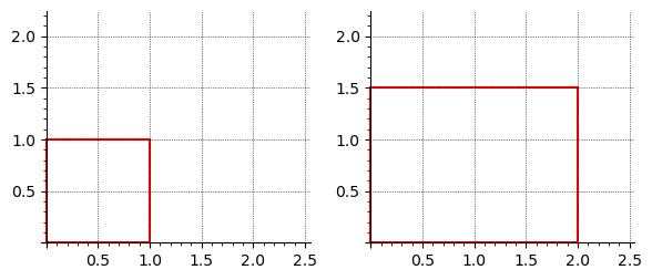
Section 3.4 Geometry of Linear Transformations

In this section, we look at some specific linear transformations from \(\R^2\) to \(R^2\) and how it transforms the unit square. Readers are encouraged to draw figures.

Subsection 3.4.1 Some special linear map from \(\R^2\to \R^2\)

Example 3.4.1. Exmpansion along \(x\)-axis..

\begin{equation*} T\left(\begin{bmatrix}x\\ y \end{bmatrix} \right)= \begin{bmatrix}ax\\y \end{bmatrix} =\begin{bmatrix}a \amp 0\\0 \amp 1 \end{bmatrix} \begin{bmatrix}x\\ y \end{bmatrix} \end{equation*}
where \(a >1\text{.}\) (Refer to the FigureΒ 3.4.2)
Figure 3.4.2. \(x\)-expansion for \(a=2\)

Example 3.4.3. Compression along \(x\)-axis..

\begin{equation*} T\left(\begin{bmatrix}x\\ y \end{bmatrix} \right)= \begin{bmatrix}ax\\y \end{bmatrix} =\begin{bmatrix}a \amp 0\\0 \amp 1 \end{bmatrix} \begin{bmatrix}x\\ y \end{bmatrix} \end{equation*}
where \(0\lt a\lt 1\text{.}\) Refer to the FigureΒ 3.4.4 for \(a=1/2\text{.}\)
Figure 3.4.4. \(x\)-Compression for \(a=1/2\)

Example 3.4.5. Expansion along \(y\)-axis.

\begin{equation*} T\left(\begin{bmatrix}x\\ y \end{bmatrix} \right)= \begin{bmatrix}x\\by \end{bmatrix} =\begin{bmatrix}0 \amp 0\\0 \amp b \end{bmatrix} \begin{bmatrix}x\\ y \end{bmatrix} \end{equation*}
where \(b>0\text{.}\) Refer to FigureΒ 3.4.6 for \(b=2\text{.}\)
Figure 3.4.6. \(y\)-expansion for \(b=2\)

Example 3.4.7. Compression along \(y\)-axis.

\begin{equation*} T\left(\begin{bmatrix}x\\ y \end{bmatrix} \right)= \begin{bmatrix}x\\by \end{bmatrix} =\begin{bmatrix}0 \amp 0\\b \amp 1 \end{bmatrix} \begin{bmatrix}x\\ y \end{bmatrix} \end{equation*}
where \(0\lt b\lt 1\text{.}\) Refer to FigureΒ 3.4.8 for \(b=1/2\text{.}\)
Figure 3.4.8. \(y\)-compression for \(b=1/2\)

Example 3.4.9. Shear along positive \(x\)-axis.

\begin{equation*} T\left(\begin{bmatrix}x\\ y \end{bmatrix} \right)= \begin{bmatrix}x+ay\\y \end{bmatrix} =\begin{bmatrix}1 \amp a\\0 \amp 1 \end{bmatrix} \begin{bmatrix}x\\ y \end{bmatrix} \end{equation*}
where \(a > 0\text{.}\) Refer to FigureΒ 3.4.10 for \(a=1/4\text{.}\)
Figure 3.4.10. Positive \(x\)-shear for \(a=1/4\)

Example 3.4.11. Shear along negative \(x\)-axis.

\begin{equation*} T\left(\begin{bmatrix}x\\ y \end{bmatrix} \right)= \begin{bmatrix}x+ay\\y \end{bmatrix} =\begin{bmatrix}1 \amp a\\0 \amp 1 \end{bmatrix} \begin{bmatrix}x\\ y \end{bmatrix} \end{equation*}
where \(a\lt 0\text{.}\) Draw the figure for \(a=-1/4\text{.}\)
Figure 3.4.12. Negative \(x\)-shear for \(a=-1/4\)

Example 3.4.13. Shear along positive \(y\)-axis.

\begin{equation*} T\left(\begin{bmatrix}x\\ y \end{bmatrix} \right)= \begin{bmatrix}x\\y+ax \end{bmatrix} =\begin{bmatrix}1 \amp 0\\a \amp 1 \end{bmatrix} \begin{bmatrix}x\\ y \end{bmatrix} \end{equation*}
where \(a > 0\text{.}\) Refer to FigureΒ 3.4.14 for \(a=1/4\text{.}\)
Figure 3.4.14. Positive \(y\)-shear for \(a=1/4\)

Example 3.4.15. Shear along negative \(y\)-axis.

\begin{equation*} T\left(\begin{bmatrix}x\\ y \end{bmatrix} \right)= \begin{bmatrix}x\\y+ax \end{bmatrix} =\begin{bmatrix}1 \amp 0\\a \amp 1 \end{bmatrix} \begin{bmatrix}x\\ y \end{bmatrix} \end{equation*}
where \(a\lt 0\text{.}\) Refer to FigureΒ 3.4.16 for \(a=-1/4\text{.}\)
Figure 3.4.16. Negative \(y\)-shear for \(a=-1/4\)

Example 3.4.17. Dilation and Contraction.

Fix a positive real number \(a\) and define \(D_a\colon \R^n\to \R^n\) by \(D_a(x)=ax\text{.}\) It is a linear map which is induced by the scalar matrix \(a I_{n}\text{.}\) ( \(D_a\) is called a dilation if \(a > 0\) and a contraction if \(a\lt 1\text{.}\)) Refer to FigureΒ 3.4.18 \(D_a\colon \R^2\to \R^2\) with \(a=2\) and \(a=1/2\text{.}\)
Figure 3.4.18. Dilations with \(a=1/4\) and \(a=2\text{.}\)

Example 3.4.19. Streching.

Let \(a\) and \(b\) be two positive real numbers and \(A=\begin{bmatrix}a \amp 0 \\0 \amp b \end{bmatrix}\text{.}\) Define \(T\colon\R^2\to \R^2\) by \(T(x)=Ax\text{.}\) Then (i) \(T\) is stretching by a factor \(a\) along \(x\)-axis and by a factor \(b\) along \(y\)-axis if \(a,b >1\) and (ii) \(T\) is contraction by a factor \(a\) along \(x\)-axis followed by a factor \(b\) along \(y\)-axis if \(0\lt a,b\lt 1\text{.}\) Refer to FigureΒ 3.4.20 for stretching along \(x\) by 2 and \(y\)-axes by 1.5.
Figure 3.4.20. Stretching along \(x\) by 2 and \(y\)-axes by 1.5.

Example 3.4.21. Geometry of linear transformation in \(\R^2\).

In this exampe, we demostrate linear transformation from \(\R^2\) to itself using the Sage interatact feature.
The follow iteract is generated using slate. You can change the input matrix and vectors and submit to see the image of vectors. Additionally, try to use the above tranformations defined such expansion, compression and shers and explore the same.
Figure 3.4.22. Goemetry of Linear Tranformation

Subsection 3.4.2 Image Tranfromation

Let us explore, how a linear transformation tranforms a grayscale image. A grayscale image is simply a 2-dimensional array (matrix) where each entry represents the intensity of light at a particular pixel. We will explain two types of transformations, scaling the intesity and rotation by an angle to a given image.
The following Python code read a grayscale image of Taj Mahal in India.
We use the transformation \(T(P)=\alpha P\text{,}\) where \(\alpha\geq 1\) is the brightness of the image. Let us take \(\alpha =1.2\) about 20/% increase in the brightness. On each pixel \(p_{ij}\) of the image \(P\text{,}\) we have \(Q=TP\text{,}\) where \(q_{ij}=\min\{\alpha p_{pij},255\}\text{.}\) Here min~255 ensures the brightness values stay within valid pixel range.
Next we plot the orginal image along with rescaled image.
Rotation Transformation
Next we apply rotation by an anngle \(30^\circ\) to this image. Note that the rotation matrix is give by
\begin{equation*} R_\theta = \begin{pmatrix} \cos \theta \amp -\sin\theta\\ \sin\theta \amp \cos\theta \end{pmatrix}. \end{equation*}

Example 3.4.23. Applying shear transform to an image.

Shear in Python is implemented as affine transformation where each point \((x, y)\) of an image is mapped to a new point \((x',y')\) via
\begin{equation*} \begin{pmatrix} x' \\ y' \\ 1 \end{pmatrix} = \begin{pmatrix} a \amp b \amp c \\ d \amp e \amp f \\ 0 \amp 0 \amp 1 \end{pmatrix} \begin{pmatrix} x \\ y \\ 1 \end{pmatrix} \end{equation*}
Hence we get
\begin{equation*} x' = a \cdot x + b \cdot y + c, \quad y' = d \cdot x + e \cdot y + f. \end{equation*}
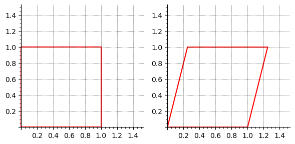
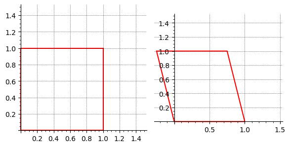
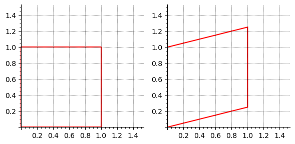
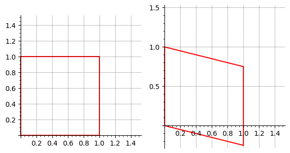
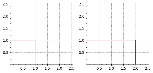
For a shear in the \(x\)-direction, we wish to shift \(x\) proportionally to \(y\) while leaving \(y\) unchanged. This corresponds to:
\begin{equation*} a = 1, \quad b = k, \quad c = 0, \quad d = 0, \quad e = 1, \quad f = 0 \end{equation*}
where \(k\) is the shear factor. Thus, the shear matrix becomes:
\begin{equation*} \begin{bmatrix} 1 \amp k \amp 0 \\ 0 \amp 1 \amp 0 \\ 0 \amp 0 \amp 1 \end{bmatrix}. \end{equation*}
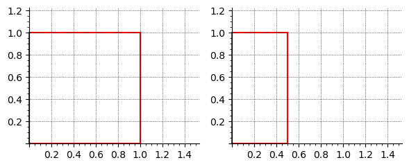
In Python’s Pillow library, the transform method uses parameters \((a, b, c, d, e, f)\) corresponding to the first two rows of the above matrix, that is,
\begin{equation*} (a, b, c, d, e, f) = (1, k, 0, 0, 1, 0). \end{equation*}

Example 3.4.24. Shear Transformation in 3D.

A shear transformation in three dimensions is a type of linear transformation that shifts one coordinate axis in proportion to another, while keeping at least one direction fixed. Unlike scaling (which stretches or compresses) or rotation (which changes orientation), shear slants the shape without changing its volume (if the determinant of the shear matrix is 1).
In matrix form, a general 3D shear is represented as
\begin{equation*} S \;=\; \begin{bmatrix} 1 \amp s_{xy} \amp s_{xz} \\ s_{yx} \amp 1 \amp s_{yz} \\ s_{zx} \amp s_{zy} \amp 1 \end{bmatrix}. \end{equation*}
Here each parameter \(s_{ij}\) determines how the \(i\)-th coordinate depends on the \(j\)-th coordinate:
  • \(s_{xy}\text{:}\) shear of \(x\)-coordinate by the \(y\)-coordinate
  • \(s_{xz}\text{:}\) shear of \(x\)-coordinate by the \(z\)-coordinate
  • \(s_{yx}\text{:}\) shear of \(y\)-coordinate by the \(x\)-coordinate
  • \(s_{yz}\text{:}\) shear of \(y\)-coordinate by the \(z\)-coordinate
  • \(s_{zx}\text{:}\) shear of \(z\)-coordinate by the \(x\)-coordinate
  • \(s_{zy}\text{:}\) shear of \(z\)-coordinate by the \(y\)-coordinate
For example, if \(s_{xy} = 1\text{,}\) then the \(x\)-coordinate increases in proportion to \(y\text{,}\) creating a slant of the cube in the \(x\)-direction depending on how far a point lies along the \(y\)-axis.
Shearing preserves parallelism of lines (parallelograms remain parallelograms, cubes become parallelepipeds) but alters angles and lengths.
In the Sage program:
  • The blue cube shows the original unit cube centered at the origin.
  • The red cube shows the sheared version after applying \(S\text{.}\)
  • Sliders let you adjust the six shear parameters and see the real-time effect.
  • The coordinate axes are drawn to help you understand the direction of shearing.
Figure 3.4.25. Shear transformation in 3d