
Section 1.1 Sytem of Linear Equation

In daily life we often encounter problems where several unknown quantities are related to each other through linear relations. Such problems naturally lead to a system of linear equations. A system of linear equations consists of several linear equations in the same set of variables. Each equation represents a constraint, and the simultaneous solution of all equations corresponds to finding the values of the unknowns that satisfy all the constraints at once.
Studying systems of linear equations is fundamental for several reasons. They arise directly in practical applicationsβ€”for instance, balancing chemical reactions, analyzing electrical networks, studying forces in equilibrium, or modeling data in statistics. Also they form the backbone of Linear Algebra, since the methods developed for their solution lead naturally to the concepts of vector spaces, linear transformations, and matrix theory.
Before moving to abstract notions of linear algebra, it is important to understand how such systems are represented, how they can be solved.
Let us start with some real life example.

Example 1.1.1.

A person travels from \(City\;A\) to \(City\;B\) using a train and a bus. The train runs at a speed of \(60\) km/h while the bus runs at \(40\) km/h. The total journey takes \(5\) hours and the total distance covered is \(240\) km. Find how much time the person spent on the train and on the bus.
Solution.
Let \(x\) be the time spent on the train (in hours), and \(y\) be the time spent on the bus (in hours). Then the problem gives us two conditions:
  1. Total travel time is \(5\) hours:
    \begin{equation*} x + y = 5. \end{equation*}
  2. Total distance is \(240\) km:
    \begin{equation*} 60x + 40y = 240. \end{equation*}
Thus the system of equations is:
\begin{equation*} \begin{cases} x + y = 5, \\ 60x + 40y = 240. \end{cases} \end{equation*}
How do we solve these equations?
From the first equation, \(y = 5 - x\text{.}\) Substituting into the second equation, we have
\begin{equation*} 60x + 40(5 - x) = 240. \end{equation*}
Simplifying this we get \(60x + 200 - 40x = 240,\text{.}\) This implies \(x = 2.\) Hence, \(y = 5 - 2 = 3.\)
Therefore, the person spent \(2\) hours on the train and \(3\) hours on the bus.
The above problem was easy to formaulate and solve. What if the problem involves more variables? Condsider the following situation now.

Example 1.1.2.

A traveler goes from \(City\;A\) to \(City\;B\) in three legs: by car at \(50\) km/h, by train at \(80\) km/h, and by ferry at \(20\) km/h. The total travel time is \(10\) hours, and the total distance covered is \(520\) km. It is also known that the time on the train equals the sume of time in the car and in ferry. Formulate this problem and fine the time (in hours) spent on each mode of transport.
Solution.
Let \(x\text{,}\) \(y\text{,}\) and \(z\) denote the hours spent by car, train, and ferry, respectively. Then the conditions give:
  1. Total time:
    \begin{equation*} x + y + z = 6. \end{equation*}
  2. Total distance:
    \begin{equation*} 50x + 80y + 20z = 520. \end{equation*}
  3. Car plus ferry time is equal to train time:
    \begin{equation*} x+z = y. \end{equation*}
Hence the linear system is
\begin{equation*} \begin{cases} x + y + z = 6,\\ 50x + 80y + 20z = 520,\\ x-y+z = 0. \end{cases} \end{equation*}
It is easy to solve the above system. It turns out that \(x = 2, y= 5\) and \(z = 3\text{.}\) Hence the traveler spends \(2\) hours by car, \(5\) hours by train, and \(3\) hours by ferry.

Example 1.1.3. Balancing Chemical Reaction Equation.

The combustion of octane (\(C_8H_{18}\)) is a classical example of a hydrocarbon fuel reacting with oxygen to form carbon dioxide and water. The unbalanced reaction is:
\begin{equation*} C_8H_{18} + O_2 \to CO_2 + H_2O. \end{equation*}
Balancing this chemical equation can be expressed as solving a system of linear equations. Let us carefully set this up for the combustion of octane:
This amounts to finding \(x,y,z,w\) such that
\begin{equation*} xC_8H_{18} + yO_2 \to zCO_2 + wH_2O. \end{equation*}
Equating the number of carbons, hydrogen and oxygen atoms on both side gives the following equations.
\begin{align*} 8x \amp=\amp z \\ 18x \amp=\amp 2w \\ 2y \amp=\amp 2z+w \end{align*}
By solving the above equations one of the soltutions is given by \(x=2, y=25, z=16, w=18 \text{.}\) Hence the balanced equation can be written as
\begin{equation*} 2C_8H_{18} + 25O_2 \to 16CO_2 + 18H_2O. \end{equation*}
Let us consider another example about distribution of taxies at various location in a certain city.

Example 1.1.4.

Consider the figure below FigureΒ 1.1.5. Vertices are various locations at which taxies are parked. The edges are directed with labels.
Figure 1.1.5. Taxi distributions between 5 locations.
For example arrow going from location 4 to 1 has label \(7/20\text{.}\) This means \(7/20^{th}=35\%\) of the taxies taken from location \(4\) comes to location \(1\) at the end of the day.
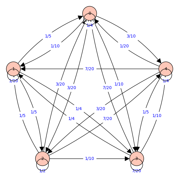
Now suppose a company is running this taxi services and has certain number of taxies. The above proportation of distribution has been otained from some past experience. Suppose the comany has a total, \(N\) taxies and wish to find out how many taxies he/she should place at various location so that his business runs smoothly. How to formulate this problem?
Suppose \(x_i\) denotes the number of taxies to be kept at the locatio \(i\text{.}\) Then we have
\begin{equation*} x_0+x_1+x_2+x_3+x_4=N. \end{equation*}
How many taxies will be there at the location \(0\) after one day. It is easy to see that it is
\begin{equation*} 1/4x_0 + 1/10x_1 + 3/20x_2 + 1/10x_3 + 3/10x_4. \end{equation*}
Similarly the number of taxies at various locations are as follows:
Ideally, the company would want the same number of taxies to come back at each location everyday. How to find these \(x_i's\text{?}\) It is easy to see that this amount to solving the following system of linear equations
\begin{align*} 1/4x_0 + 1/10x_1 + 3/20x_2 + 1/10x_3 + 3/10x_4\amp =\amp x_0\\ 1/5x_0 + 1/10x_1 + 1/5x_2 + 1/4x_3\amp =\amp x_1\\ 3/20x_0 + 1/5x_1 + 1/2x_2 + 1/10x_3 + 7/20x_4 \amp =\amp x_1\\ 7/20x_0 + 1/4x_1 + 7/20x_3 + 1/10x_4\amp= \amp x_3\\ 1/20x_0 + 7/20x_1 + 3/20x_2 + 1/5x_3 + 1/4x_4\amp =\amp x_4 \end{align*}
The above equations can be written in a matrix form as follows:
\begin{equation*} \left(\begin{array}{rrrrr} \frac{1}{4} \, x_{0} + \frac{1}{10} \, x_{1} + \frac{3}{20} \, x_{2} + \frac{1}{10} \, x_{3} + \frac{3}{10} \, x_{4} \\ \frac{1}{5} \, x_{0} + \frac{1}{10} \, x_{1} + \frac{1}{5} \, x_{2} + \frac{1}{4} \, x_{3} \\ \frac{3}{20} \, x_{0} + \frac{1}{5} \, x_{1} + \frac{1}{2} \, x_{2} + \frac{1}{10} \, x_{3} + \frac{7}{20} \, x_{4} \\ \frac{7}{20} \, x_{0} + \frac{1}{4} \, x_{1} + \frac{7}{20} \, x_{3} + \frac{1}{10} \, x_{4} \\ \frac{1}{20} \, x_{0} + \frac{7}{20} \, x_{1} + \frac{3}{20} \, x_{2} + \frac{1}{5} \, x_{3} + \frac{1}{4} \, x_{4} \end{array}\right) = \left(\begin{array}{rrrrr} x_{0} \\ x_{1} \\ x_{2} \\ x_{3} \\x_{4} \end{array}\right). \end{equation*}
The above equation can be written as
\begin{equation*} \left(\begin{array}{rrrrr} \frac{1}{4} \amp \frac{1}{10} \amp \frac{3}{20} \amp \frac{1}{10} \amp \frac{3}{10} \\ \frac{1}{5} \amp \frac{1}{10} \amp \frac{1}{5} \amp \frac{1}{4} \amp 0 \\ \frac{3}{20} \amp \frac{1}{5} \amp \frac{1}{2} \amp \frac{1}{10} \amp \frac{7}{20} \\ \frac{7}{20} \amp \frac{1}{4} \amp 0 \amp \frac{7}{20} \amp \frac{1}{10} \\ \frac{1}{20} \amp \frac{7}{20} \amp \frac{3}{20} \amp \frac{1}{5} \amp \frac{1}{4} \end{array}\right) \left(\begin{array}{rrrrr} x_{0} \\ x_{1} \\ x_{2} \\ x_{3} \\x_{4} \end{array}\right)=\left(\begin{array}{rrrrr} x_{0} \\ x_{1} \\ x_{2} \\ x_{3} \\x_{4} \end{array}\right). \end{equation*}
We can write it in compact form as \(AX=X\) where
\begin{equation*} A = \left(\begin{array}{rrrrr} \frac{1}{4} \amp \frac{1}{10} \amp \frac{3}{20} \amp \frac{1}{10} \amp \frac{3}{10} \\ \frac{1}{5} \amp \frac{1}{10} \amp \frac{1}{5} \amp \frac{1}{4} \amp 0 \\ \frac{3}{20} \amp \frac{1}{5} \amp \frac{1}{2} \amp \frac{1}{10} \amp \frac{7}{20} \\ \frac{7}{20} \amp \frac{1}{4} \amp 0 \amp \frac{7}{20} \amp \frac{1}{10} \\ \frac{1}{20} \amp \frac{7}{20} \amp \frac{3}{20} \amp \frac{1}{5} \amp \frac{1}{4} \end{array}\right) \quad \text{and} \quad X=\left(\begin{array}{rrrrr} x_{0} \\ x_{1} \\ x_{2} \\ x_{3} \\x_{4} \end{array}\right). \end{equation*}

Question 1.1.6.

In the ExampleΒ 1.1.4, suppose we denote \(AX\) by \(X_1\text{,}\) then \(X_1\) is the number of taxies at various locations. What will the the number taxies after two days, three days and in general after \(n\) days.

Remark 1.1.7.

Note that the preoblem in ExampleΒ 1.1.4 involves only 5 depos. What if we have hundreds of depos? How do we solve such problems? In fact, google seach uses millions by million equations. It turns out that solving this problem amounts to finding large power of the coefficient matrix \(A\) whihc is not an easy task even for poweful computers. This is acheived by notion of diagonalization whihc and numerical computaions of eigenvalues and eigenvectors of a large size matrix. We shall see several such applications in later chapters.
Let us define what is meaning of a system of linear equations involving certain variables. Think about the following questions before making a formal definition of system of linear equations.

Question 1.1.8.

How will you write one linear equation involving 20 variables? May be you can name the variables \(x, y,z,\alpha, \beta \) etc
How will you write one linear equation involving as many variables as number of active websites, say \(n\) on this date?
How will you write \(\) linear equations in \(n\) variables where \(n\) when \(m\) and \(n\) are very large?
The above series of questions leads to requirement of double indexing for defining a system of linear equations.

Definition 1.1.9.

A system of linear equations is a finite collection of linear equations. Consider a system of \(m\) linear equations in \(n\)-variables \(x_1,\ldots, x_n\text{.}\)
\begin{align} a_{11}x_1 + a_{12}x_2+ \ldots + a_{1n} x_n \amp= \amp b_1\notag\\ a_{21}x_1 + a_{22}x_2+ \ldots + a_{2n} x_n \amp= \amp b_2\notag\\ \vdots \amp \amp \vdots \tag{1.1.1}\\ a_{m1}x_1 + a_{m2}x_2+ \ldots + a_{mn} x_n \amp = \amp b_m\notag \end{align}
Here \(a_{ij}\in \R\) for \(1\leq i\leq m,1\leq j\leq n\) and \(b_i\in \R\) for \(1\leq i\leq m\text{.}\)
The above system of linear equations can be represented in compact form using the summation notation as follows:
\begin{equation} \sum_{j=1}^n a_{ij}x_j =b_i,\quad 1\leq i\leq m\text{.}\tag{1.1.2} \end{equation}
Next let us define, what is meaning of a solution and the solution set of the system of linear of equations (1.1.1).

Definition 1.1.10.

A solution of the system of linear equations (1.1.1) is an ordered \(n\)-tuple of the real numbers \((y_1, y_2, \cdots, y_n)\) such that \(x_i = y_i\) for each \(i = 1, 2, \ldots, n\) satisfies each of the \(m\)-equations. The set of all solutions of a system is called the solution set. It is a subset of \(\R^n\text{,}\) the Cartesian product of the set \(\R\) of real numbers \(n\)-times. If we denote the solution set by \(S\text{,}\) then
\begin{equation*} S=\{(x_1,\ldots,x_n)\in \R^n:\sum_{j=1}^n a_{ij}x_j =b_i,\quad 1\leq i\leq m\}\text{.} \end{equation*}
If the solution set is nonempty then the system is said to be consistent and otherwise it is said to be inconsistent.
The above system of linear equation can be written as a single matrix equation as
\begin{equation} AX = B\text{,}\tag{1.1.3} \end{equation}
where
\begin{equation} A=\begin{pmatrix} a_{11} \amp a_{12} \amp \ldots \amp a_{1n} \\ a_{21} \amp a_{22} \amp \ldots \amp a_{2n} \\ \vdots\amp \vdots\amp \vdots\amp \vdots\\ a_{m1} \amp a_{m2} \amp \ldots \amp a_{mn} \end{pmatrix}, \quad X=\begin{pmatrix}x_1\\x_2\\ \vdots\\ x_n \end{pmatrix}, \quad B=\begin{pmatrix}b_1\\b_2\\ \vdots\\ b_m \end{pmatrix}. \tag{1.1.4} \end{equation}
The matrix \(A\) is called the coefficient matrix, \(B\) is called the column matrix of constants or known terms and \(X\) is called the column matrix of the unknowns.
All the essential data of the system can be gathered in one matrix by inserting the column matrix of the constants to the coefficient matrix as \(n+1\)-th column. This matrix is called the augmented or enlarged matrix of the system. Once we know the system, we can get the augmented matrix associated with the system and conversely once we know the augmented matrix, we know the system and start calculating the solutions.
The augmented matrix of the above system \(AX=B\) is given by
\begin{equation} [A~|~B]= \begin{pmatrix} a_{11} \amp a_{12} \amp \cdots \amp a_{1n} \amp | \amp b_1\\ a_{21} \amp a_{22} \amp \cdots \amp a_{2n} \amp | \amp b_2\\ \vdots \amp \vdots \amp \ddots \amp \vdots \amp \vdots \amp \vdots\\ a_{m1} \amp a_{m2} \amp \cdots \amp a_{mn} \amp | \amp b_m\\ \end{pmatrix}.\tag{1.1.5} \end{equation}

Definition 1.1.11.

Two systems of linear equations are called equivalent if and only if they have the same set of solutions.
We will define some basic operations by which a system is transformed into an equivalent system.
Geometrically, solving a system of linear equations in two (or three) unknowns/variables is equivalent to determining whether or not a family of lines (or planes) has a common point of intersection.

Remark 1.1.12.

Let \(A\) be \(n\times n\) real matrix whose columns are \(a_1,\ldots, a_n\) and \(x=\begin{pmatrix}x_1\amp\cdots \amp x_n\end{pmatrix}^T\text{.}\) Then
\begin{equation*} Ax=x_1a_1+x_2a_2+\cdots +a_nx_n. \end{equation*}
In particular, \(Ax\) is a linear combinations of column of \(A\text{.}\) Thus if \(\alpha=\begin{pmatrix}\alpha_1\amp\cdots \amp \alpha_n\end{pmatrix}^T\) is a solution of \(Ax=b\text{,}\) then \(b\) is linear combination of columns of \(A\text{.}\) For example,
\begin{equation*} AX= \begin{pmatrix} 2 \amp 3 \amp 1 \amp 4\\ 1 \amp 2 \amp -1 \amp 3\\ 3 \amp -2 \amp 0 \amp 2\\ -2 \amp 0 \amp 2 \amp 1 \end{pmatrix} \begin{pmatrix} x_1\\x_2\\x_3\\x_4\end{pmatrix} =\begin{pmatrix} 2 x_1+ 3x_2 + x_3 + 4x_4\\ x_1 +2x_2 -x_3+ 3x_3\\ 3 x_1 -2 x_2+2x_4\\ -2x_1 + 2x_3 +x_4 \end{pmatrix}. \end{equation*}
This can be written as
\begin{equation*} AX= x_1 \begin{pmatrix} 2\\1\\3\\-2\end{pmatrix}+ x_2 \begin{pmatrix} 3\\2\\-2\\0\end{pmatrix}+ x_3 \begin{pmatrix} 1\\-1\\0\\2\end{pmatrix}+ x_4 \begin{pmatrix} 4\\3\\2\\1\end{pmatrix}. \end{equation*}
Our goal in this chapter is to find the solution set \(S\) of a system of equations \(Ax=b\text{.}\) Let us first find solution set involving one equation involving one and two variables.

Example 1.1.13.

One linear equation in one variable \(x\) can be written as
\begin{equation} ax =b,\tag{1.1.6} \end{equation}
where, \(a\) and \(b\) are real numbers.
How to find the solution set of this equation. We need to find \(x\in\R\) such that the equation holds. Does it mean \(x=b/a\text{?}\) What if \(a=0\text{?}\) Thus we need to consider different cases on \(a\text{.}\) If \(S\) is the solution set of this equation then we have
\begin{equation*} S = \begin{cases} \emptyset, \amp \text{ if } a=0\\ \R, \amp \text{ if } a=0, b=0\\ \{b/a\}, \amp \text{ if } a\neq 0\\ \end{cases}. \end{equation*}

Example 1.1.14.

One linear equation in two variable \(x\) and \(y\) can be written as
\begin{equation} ax+by =c,\tag{1.1.7} \end{equation}
where, \(a, b\) and \(c\) are real numbers. How to find the solution set \(S\) of this equation?
Solution.
In this case, we need to consider two cases: (i) \(a=0=b\) and (ii) at least one of \(a, b \)is nonzero. If \(a=0=b\text{,}\) then the solution depends upon \(c\text{.}\) If \(c=0\text{,}\) then \(S=\R\) and if \(c\neq 0\text{,}\) then \(S=\emptyset\text{,}\) the empty/null set.
In the second case, the solution set has geometric interpretation, it is that the set of all points on a straight line. For example, if \(b\neq 0\text{,}\) then the set of solutions is the straight line in the plane through the point \((0,c/b)\) and with slope \(-a/b\text{.}\) If \(b=0\text{,}\) then also the solution set is a straight line. Can you identify it?
Can you write the solution set explicitley by taking all the possible cases?

Remark 1.1.15.

The solution set of one linear equation \(ax+by=c\text{,}\) where \(a,b,c\in \R\) in two variables is a straight line provides \((a,b)\neq (0,0)\text{,}\) that is, one of the coefficients \(a\) or \(b\) is non-zero.

Question 1.1.16.

Write the solution set of tne linear equation in three variables \(ax+by+cz=d\text{,}\) where \(a,b,c,d\in\R\text{.}\)

Remark 1.1.17.

Let at least one of the \(a,b, c\text{,}\) be nonzero, the solution set \(S=\{(x,y,z)\in\R^3: ax+by+cz=d\}\) is a plane in \(\R^3\text{.}\)